pipeline latency

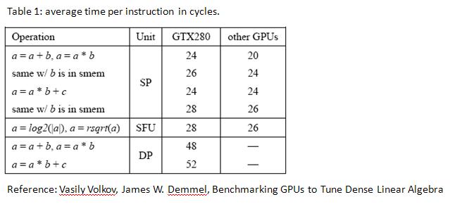
In paper [1], authors measure pipeline latency on several graphic card and reports in table 1.

table 1, pipeline_latency_table.jpg

[img]http://oz.nthu.edu.tw/~d947207/NVIDIA/pipeline_latency/pipeline_latency_table.JPG[/img]

the table shows that register-to-register MAD (multiply-and-add) instruction runs at 24 cycles.

and authors argue "24 cycle latency may be hidden by running simultaneously 6 warps (or 192 threads) per SM".

this match description section 5.1.2.6 n programming guide,

"Generally, accessing a register is zero extra clock cycles per instruction, but delays may occur due to register read-after-write dependencies and register memory bank conflicts.

The delays introduced by read-after-write dependencies can be ignored as soon as there are at least 192 active threads per multiprocessor to hide them"

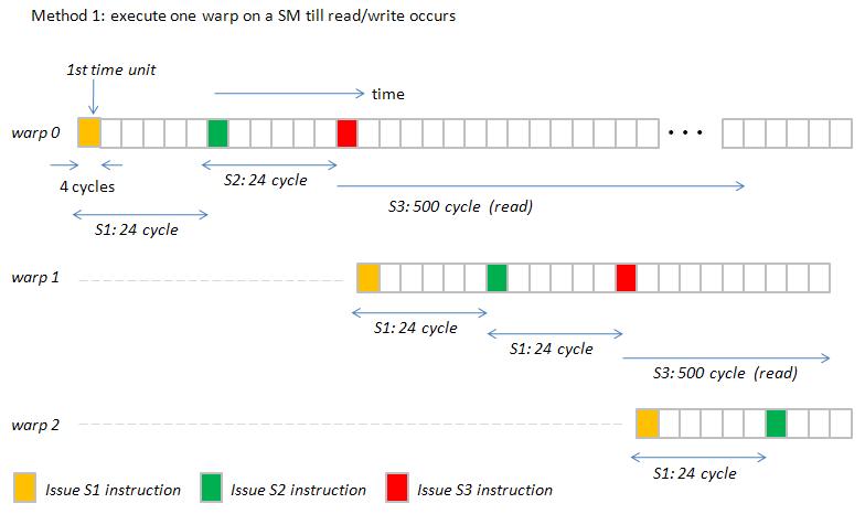
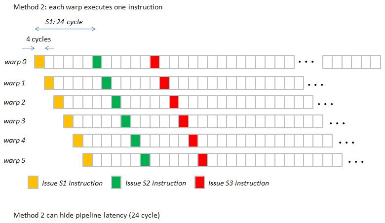
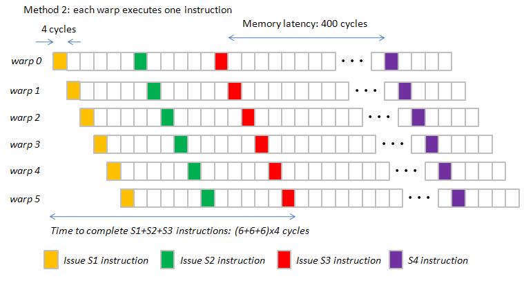
Question: how does scheduler dispatch warps in a SM? Two methods,

Method 1 :  Warp occupies SPs till memory-access instruction is executed.

Method 2 :  Each warp execute one instruction in turn.

In section 4.1 of programming guide, it says “Every instruction issue time, the SIMT unit selects a warp that is ready to execute and issues the next instruction to the active threads of the warp”.

It seems that hardware supports method 2.

I take an example to show method 1 and method 2.

Example :  execute three instructions S1, S2 and S3 in turn

[code]

S1 : a ß a * b + c     ; // register read-after-write dependence

S2 : a ß a * b + c    ; // register read-after-write dependence

S3 : odata[index] ß a    ;// read operation

[/code]

we show Gatt chart of method 1 in figure 1 and Gatt chart of method 2 in figure 2.

figure 1, pipeline_latency_1.jpg

[img]http://oz.nthu.edu.tw/~d947207/NVIDIA/pipeline_latency/pipeline_latency_1.JPG[/img]

figure 2, pipeline_latency_2.jpg

[img]http://oz.nthu.edu.tw/~d947207/NVIDIA/pipeline_latency/pipeline_latency_2.JPG[/img]

Reference: [1] Vasily Volkov, James W. Demmel, Benchmarking GPUs to Tune Dense Linear Algebra

=======================================================================================

Although method 2 is right, but it is tedious to draw Gatt chart under method 2.

I don’t adopt method 2 to draw Gatt chart when compare bandwidth between “float” and “double” in the thread

http://forums.nvidia.com/index.php?showtopic=106924&pid=600634&mode=threaded&start=#entry600634.

In that topic, I don’t use pipeline latency but calibrate “index computation” via Block-wise test harness provided by SPWorley.

in the thread http://forums.nvidia.com/index.php?showtopic=103046 , @SPWorley uses one block of 192 threads to calibrate

"how many clocks the operation takes".

following code is kernel of calibration.

[code]

#define ITEST(num) \

ikernel<itest_ ## num, EVALLOOPS> <<<1,192>>>(12345, d_result); \

cudaMemcpy( &h_result, d_result, sizeof(int), cudaMemcpyDeviceToHost); \

printf("I" #num " %4.1lf %s\n", \

itest_ ## num ().describe());

[/code]

@SPWorley's code uses

(1) 192 threads to hide pipeline latency and

(2) unroll large loop

Question: what is relationship between pipeline latency and SPWorley uses one block of 192 threads to calibrate “how many clocks it takes”.

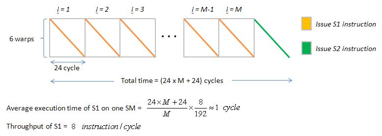
first suppose we want to evaluate operation S1 ( a <-- a * b + c ), then  we must do S1 large times, say M times.

[code]

for  i = 1: M

    S1 : a <-- a * b + c     ; // register read-after-write dependence

end

S2 : a <-- a * b + c    ; // register read-after-write dependence

[/code]

Then it is easy to plot Gatt chart of above code, just modify Gatt chart in figure 2, repeat operation S1 M times , see figure 3.

figure 3, pipeline_latency_3.jpg

[img]http://oz.nthu.edu.tw/~d947207/NVIDIA/pipeline_latency/pipeline_latency_3.JPG[/img]

if M is large enough, then average execution time of S1 on one SM is about 1 cycle. (when all 8 SP executes S1 simultaneously, it only needs 1 cycle to complete S1)

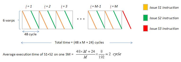
similarly if we want to calibrate operation "S1 + S2" in the following code,

[code]

for i = 1: M

   S1 : a  <-- a * b + c     ; // register read-after-write dependence

   S2 : a  <-- a * b + c    ; // register read-after-write dependence

end

S3 : odata[index]  <-- a    ; // write operation

[/code]

then Gatt chart is figure 4. average execution time of S1+S2 on one SM is about 2 cycle

figure 4, pipeline_latency_4.jpg

[img]http://oz.nthu.edu.tw/~d947207/NVIDIA/pipeline_latency/pipeline_latency_4.JPG[/img]

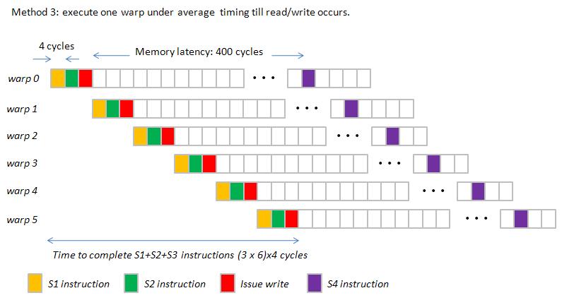
Average execution time of S1 on one SM = 1 cycle, this means that one warp needs 4 cycle to execute S1 instruction

in average sense. We define method 3 as method 1 but with average execution time of instructions.

Then Gatt chart of following code is figure 5

[code]

//Example :  execute three instructions S1, S2 and S3 in turn

S1 : a <-- a * b + c     ; // register read-after-write dependence

S2 : a <-- a * b + c    ; // register read-after-write dependence

S3 : odata[index] <-- a    ; // write operation

S4:  a <--  a * b + c  ;

[/code]

figure 5, pipeline_latency_5.jpg

[img]http://oz.nthu.edu.tw/~d947207/NVIDIA/pipeline_latency/pipeline_latency_5.JPG[/img]

however if we use method 2, then Gatt chart is figure 6

figure 6, pipeline_latency_6.jpg

[img]http://oz.nthu.edu.tw/~d947207/NVIDIA/pipeline_latency/pipeline_latency_6.JPG[/img]

Observation: difference between method 2 and method 3

(1) Method 3 hides "index computation" in memory latency while method 2 hide "index computation" in pipeline latency. 

(2) Space between two read/write operation (red rectangle) is larger in method 3.

However critical timing of method 2 and method 3 are the same, so we can use method 3 to plot Gatt chart.

To sum up, I think that it is reasonable to draw Gatt chart by method 3, which is more simple.